Built-In Variants

The classes in ddtw.ddtw_variants are convenience frontends around the general dDTW class. Each variant fixes the graph components introduced in the core concepts:

\[\mathcal{S},\qquad \mathbf{W},\qquad \mathcal{B}_\mathrm{start},\qquad \mathcal{B}_\mathrm{end},\qquad \mu.\]

The table uses the paper’s one-based notation. Tensor indices in the implementation are zero-based.

Parameter Overview

Variant	\(\mathcal{S}\)	\(\mathbf{W}(n,m)\)	\(\mathcal{B}_\mathrm{start}\)	\(\mathcal{B}_\mathrm{end}\)	\(\mu\)
DTW SDTW smoothDTW sparseDTW	\((1,0)\) \((0,1)\) \((1,1)\)	\([1,1,1]\)	\(\{(1,1)\}\)	\(\{(N,M)\}\)	\(\mu_\mathrm{hard}\) \(\mu_\mathrm{soft}\) \(\mu_\mathrm{smooth}\) \(\mu_\mathrm{sparse}\)
subSDTW	\((1,0)\) \((0,1)\) \((1,1)\)	\([1,1,1]\)	\((1,1),\ldots\) \((N,1)\)	\((1,M),\ldots\) \((N,M)\)	\(\mu_\mathrm{hard}\) or \(\mu_\mathrm{soft}\)
partial_matching	\((1,0)\) \((0,1)\) \((1,1)\)	\([0,0,1]\)	\(\mathcal{I}\)	\(\mathcal{I}\)	\(\mu_\mathrm{hard}\) or differentiable \(\mu\)
CTC	\((1,0)\) \((1,1)\) \((1,2)\)	allowed: \([1,1,1]\) forbidden skip: \([1,1,\infty]\)	\((1,1)\) \((1,2)\)	\((N,2M)\) \((N,2M+1)\)	\(\mu_\mathrm{soft}\)

DTW and Differentiable DTW Variants

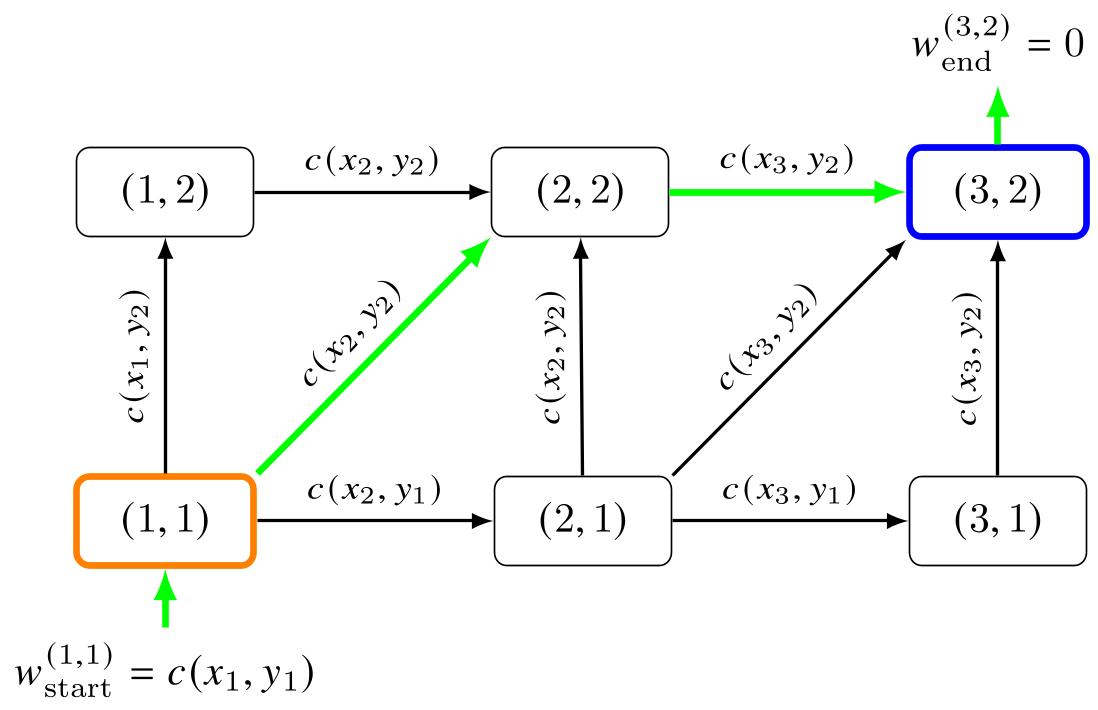
Classical DTW and SDTW use the same graph topology. [1] [2]

\[\mathcal{S}=\{(1,0),(0,1),(1,1)\},\qquad \mathbf{W}(n,m)=[1,1,1],\]

with boundary conditions

\[\mathcal{B}_\mathrm{start}=\{(1,1)\},\qquad \mathcal{B}_\mathrm{end}=\{(N,M)\}.\]

They differ only in the aggregation operator. DTW uses \(\mu_\mathrm{hard}\), so it selects one minimum-cost path. SDTW uses \(\mu_\mathrm{soft}\), so it softly aggregates all paths and yields a smooth loss. The start weight \(w_\mathrm{start}^{(1,1)}=c(x_1,y_1)\) accounts for the initial local cost, and \(w_\mathrm{end}^{(N,M)}=0\).

smoothDTW and sparseDTW keep the same graph and boundary conditions but replace \(\mu\) by \(\mu_\mathrm{smooth}\) or \(\mu_\mathrm{sparse}\). [3] [4] These operators can be used as differentiable recursive losses, but they do not yield the same global path aggregation cost guaranteed for hardmin and softmin.

Subsequence (S)DTW

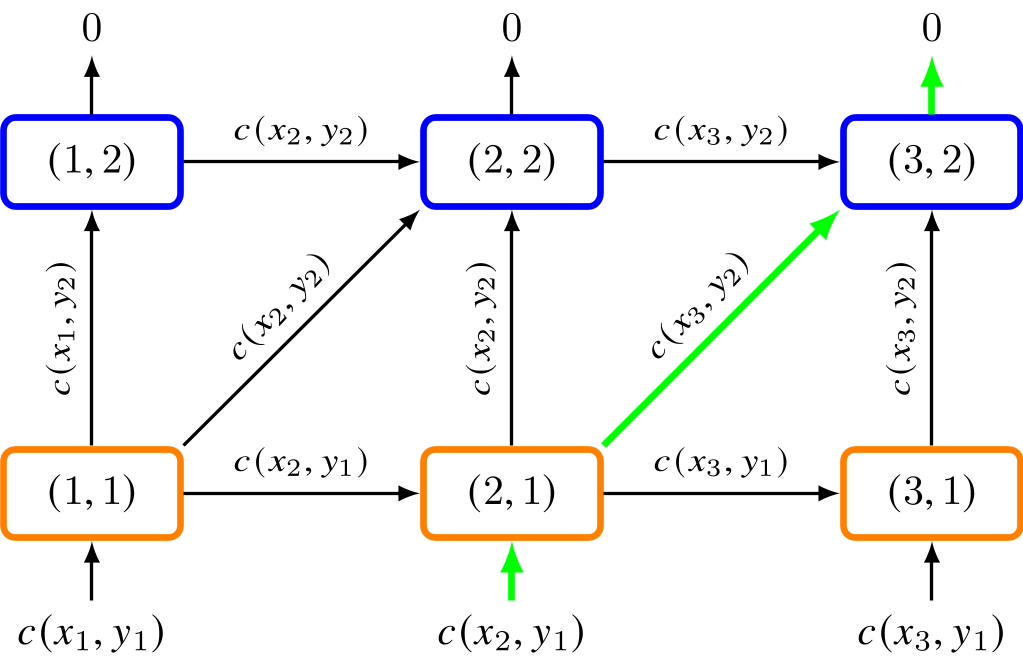
subSDTW is designed for matching a query sequence \(Y=(y_1,\ldots,y_M)\) to a subsequence of a longer document \(X=(x_1,\ldots,x_N)\), typically with \(N\gg M\). [5] It keeps the standard DTW step set

\[\mathcal{S}=\{(1,0),(0,1),(1,1)\}\]

but widens the boundary conditions. For the standard query-in-document setup, paths may start anywhere in the first query column and end anywhere in the last query column:

\[\mathcal{B}_\mathrm{start} = \{(1,1),\ldots,(N,1)\}, \qquad \mathcal{B}_\mathrm{end} = \{(1,M),\ldots,(N,M)\}.\]

Hard subsequence DTW uses \(\mu_\mathrm{hard}\); differentiable subsequence SDTW uses \(\mu_\mathrm{soft}\). [6] The toolbox also exposes boundary penalties. These implement the idea that start and end weights can compensate for skipped prefixes or suffixes and help prevent collapse to overly short alignments.

In the implementation, sub_X and sub_Y control whether subsequence behavior is enabled along the prediction axis, the target axis, or both.

Partial Matching

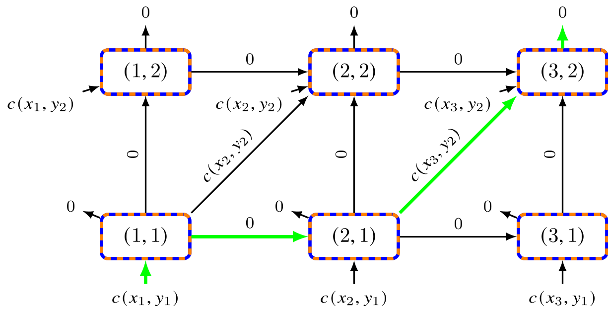
Partial matching selects a monotonically ordered subset of matched sequence elements. [7] [8] [9] This behavior is obtained by keeping the standard step set

\[\mathcal{S}=\{(1,0),(0,1),(1,1)\}\]

but assigning zero weight to horizontal and vertical moves:

\[\mathbf{W}(n,m)=[0,0,1].\]

Only diagonal steps accumulate the local matching cost. Since the match may start and end anywhere,

\[\mathcal{B}_\mathrm{start} = \mathcal{B}_\mathrm{end} = \mathcal{I}.\]

The local cost \(c\) should encode whether a local correspondence is favorable. In the classical formulation, favorable matches have negative costs and unfavorable matches have positive costs, so the best path selects a useful ordered subset. The toolbox default partial_matching class uses cost_function="CTC" and min_function="hardmin", but the same graph can be paired with differentiable minimum functions when a smooth approximation is desired.

CTC

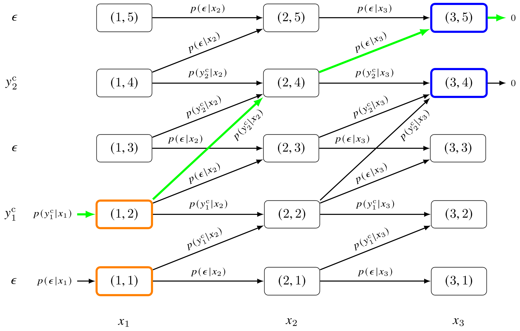
CTC is represented by expanding the target sequence with the blank symbol \(\epsilon\): [10] [11]

\[Y^\mathrm{e} = (\epsilon,y_1,\epsilon,\ldots,y_M,\epsilon).\]

The alignment graph is then built over \(X\) and \(Y^\mathrm{e}\). The local cost is the negative log-probability

\[c(x_n,y_m^\mathrm{e}) = -\log p(y_m^\mathrm{e}\mid x_n).\]

Paths start either at the initial blank or at the first target symbol and end either at the final target symbol or at the final blank:

\[\mathcal{B}_\mathrm{start} = \{(1,1),(1,2)\}, \qquad \mathcal{B}_\mathrm{end} = \{(N,2M),(N,2M+1)\}.\]

The step set is

\[\mathcal{S}=\{(1,0),(1,1),(1,2)\}.\]

All steps are strictly monotonic in \(n\), so each input frame is consumed in order. A \((1,2)\) step skips over a blank and is allowed only when the adjacent target labels differ. The toolbox implements this constraint through local step weights

\[\mathbf{W}\in\{1,\infty\}^{N\times(2M+1)\times3},\]

where finite weights mark allowed transitions and infinite weights suppress forbidden blank-skipping or repeated-label transitions. The aggregation operator is \(\mu_\mathrm{soft}\), which recovers the usual CTC log-sum-exp over valid label paths within the dDTW graph formulation.

In code, pass log-probabilities as X and integer target labels as Y. The class constructs \(Y^\mathrm{e}\), boundary sets, and local transition weights automatically.

References

[1]

M. Muller, Fundamentals of Music Processing: Using Python and Jupyter Notebooks, 2nd ed. Springer, 2021.

[2]

M. Cuturi and M. Blondel, “Soft-DTW: a Differentiable Loss Function for Time-Series,” in Proceedings of the International Conference on Machine Learning (ICML), Sydney, NSW, Australia, 2017, pp. 894-903.

[3]

I. Hadji, K. G. Derpanis, and A. D. Jepson, “Representation Learning via Global Temporal Alignment and Cycle-Consistency,” in Proceedings of the IEEE/CVF Conference on Computer Vision and Pattern Recognition (CVPR), Virtual, 2021, pp. 11068-11077.

[4]

A. Mensch and M. Blondel, “Differentiable Dynamic Programming for Structured Prediction and Attention,” in Proceedings of the International Conference on Machine Learning (ICML), Stockholm, Sweden, 2018, pp. 3459-3468.

[5]

S. Balke, V. Arifi-Muller, L. Lamprecht, and M. Muller, “Retrieving Audio Recordings Using Musical Themes,” in Proceedings of the IEEE International Conference on Acoustics, Speech, and Signal Processing (ICASSP), Shanghai, China, 2016, pp. 281-285.

[6]

J. Zeitler and M. Muller, “Subsequence SDTW: Differentiable Alignment with Flexible Boundary Conditions,” in Proceedings of the IEEE International Conference on Acoustics, Speech, and Signal Processing (ICASSP), Barcelona, Spain, 2026.

[7]

P. A. Pevzner, Computational Molecular Biology: An Algorithmic Approach. MIT Press, 2000.

[8]

M. Muller and D. Appelt, “Path-Constrained Partial Music Synchronization,” in Proceedings of the IEEE International Conference on Acoustics, Speech, and Signal Processing (ICASSP), Las Vegas, Nevada, USA, 2008, pp. 65-68.

[9]

S. Ewert, M. Muller, V. Konz, D. Mullensiefen, and G. A. Wiggins, “Towards Cross-Version Harmonic Analysis of Music,” IEEE Transactions on Multimedia, vol. 14, no. 3-2, pp. 770-782, 2012.

[10]

A. Graves, S. Fernandez, F. J. Gomez, and J. Schmidhuber, “Connectionist Temporal Classification: Labelling Unsegmented Sequence Data with Recurrent Neural Networks,” in Proceedings of the International Conference on Machine Learning (ICML), Pittsburgh, Pennsylvania, USA, 2006, pp. 369-376.

[11]

J. Zeitler and M. Muller, “A Unified Perspective on CTC and SDTW Using Differentiable DTW,” IEEE Transactions on Audio, Speech and Language Processing, vol. 34, pp. 936-951, 2026.