Core Concepts

The following introduction to the dDTW graph is based on concepts introduced by Mensch & Blondel [2] and Zeitler & Müller. [6]

dDTW models monotonic sequence alignment as path-cost aggregation on a weighted directed acyclic graph. The presented theory is expressed in one-based notation, matching the paper. The toolbox uses zero-based tensor indices internally, so a paper vertex \((1, 1)\) is represented by index [0, 0] in code. [1]

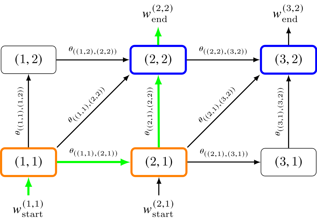
Example alignment graph with \(\mathcal{I}=[1{:}3]\times[1{:}2]\), \(\mathcal{S}=\{(1,0),(0,1),(1,1)\}\), start vertices \(\mathcal{B}_\mathrm{start}=\{(1,1),(2,1)\}\), end vertices \(\mathcal{B}_\mathrm{end}=\{(2,2),(3,2)\}\), and one highlighted path.

Definition of the Alignment Graph

Let

\[X=(x_1,\ldots,x_N),\qquad Y=(y_1,\ldots,y_M)\]

be two sequences with elements \(x_n\in\mathcal{F}_X\) and \(y_m\in\mathcal{F}_Y\). In general, we assume \(X\) to be a sequence of DNN predictions and \(Y\) a sequence of training targets. In the toolbox, we represent these sequences as torch.tensor objects with shapes (B,N,D) and (B,M,D), respectively, where B denotes batch size, N and M denote sequence lengths, and D denotes feature dimensions.

The alignment graph is specified by vertices, directed edges, edge weights, boundary conditions, and the paths induced by these choices.

Vertices

Temporal correspondences \((x_n,y_m)\) are represented by vertices \(p=(n,m)\) on the grid

\[\mathcal{I}:= [1{:}N]\times[1{:}M].\]

Thus, every vertex corresponds to one possible local pairing between the two sequences.

Edges

Allowed alignment steps are collected in

\[\mathcal{S}:= \{(i_s,j_s)\mid s\in[1{:}S]\}\subset\mathbb{N}_0^2, \qquad i_s+j_s\geq 1.\]

They induce directed edges

\[\mathcal{E}:= \{(p',p)\in\mathcal{I}^2\mid p-p'\in\mathcal{S}\}.\]

Because every step increases at least one index, the graph \((\mathcal{I},\mathcal{E})\) is acyclic and can be evaluated in topological order. [2] In the toolbox, \(\mathcal{S}\) is defined via the variable step_sizes as a list of tuples [[i_1,j_1], ..., [i_S,j_S]].

Edge Weights

A local cost function

\[c:\mathcal{F}_X\times\mathcal{F}_Y\rightarrow\mathbb{R}\]

quantifies the dissimilarity between sequence elements. In the toolbox, cost functions can be selected from ("MSE", "BCE", "CTC"), where the latter denotes the inner product between its inputs. Optional step weights

\[\mathbf{W}\in\mathbb{R}^{N\times M\times S}\]

modify the cost depending on the cell \((n,m)\) and incoming step \(s\). For an edge \((p',p)\) with \(p=(n,m)\) and \(p-p'=(i_s,j_s)\), the edge weight is

\[\theta_{(p',p)} := c(x_n,y_m)\cdot\mathbf{W}(n,m,s).\]

The toolbox exposes constant step weights through a list of global_step_weights=[w_1, ..., w_S], which define the same set of step weights for all cells. Cell-dependent weights are set through local_step_weights as a torch.tensor with shape (B,N,M,S).

Boundary Conditions

The allowed start and end vertices are sets

\[\mathcal{B}_\mathrm{start},\mathcal{B}_\mathrm{end}\subseteq\mathcal{I}.\]

In the toolbox, these are implemented as a list of lists [[start_vertices_batch_1], ..., [start_vertices_batch_B]] and [[end_vertices_batch_1], ..., [end_vertices_batch_B]]. Additional boundary weights \(w_\mathrm{start}^p\) and \(w_\mathrm{end}^p\) define costs for selected start and end vertices. These weights are useful, for example, when the cost of subsequence alignments should be compensated for the skipped prefix or suffix. In the toolbox, the weights are implemented as lists of multiplicative weights [[start_weights_batch_1], ..., [start_weights_batch_B]] and [[end_weights_batch_1], ..., [end_weights_batch_B]], where the list lengths must correspond to B_start, B_end.

Paths

A path \((p_1,\ldots,p_L)\in\mathcal{I}^L\) is a sequence of vertices connected by edges \((p_{\ell-1},p_\ell)\in\mathcal{E}\). Every valid path starts at \(p_1\in\mathcal{B}_\mathrm{start}\). A full alignment path also ends at \(p_L\in\mathcal{B}_\mathrm{end}\). For a vertex \(p\in\mathcal{I}\), let \(\mathcal{P}(p)\) denote all paths starting in \(\mathcal{B}_\mathrm{start}\) and ending at \(p\).

Graph-Based Alignment Cost

The graph specifies which alignments are possible. The aggregation operator specifies how the costs of all possible paths are combined into one loss.

Cost Aggregation Operators

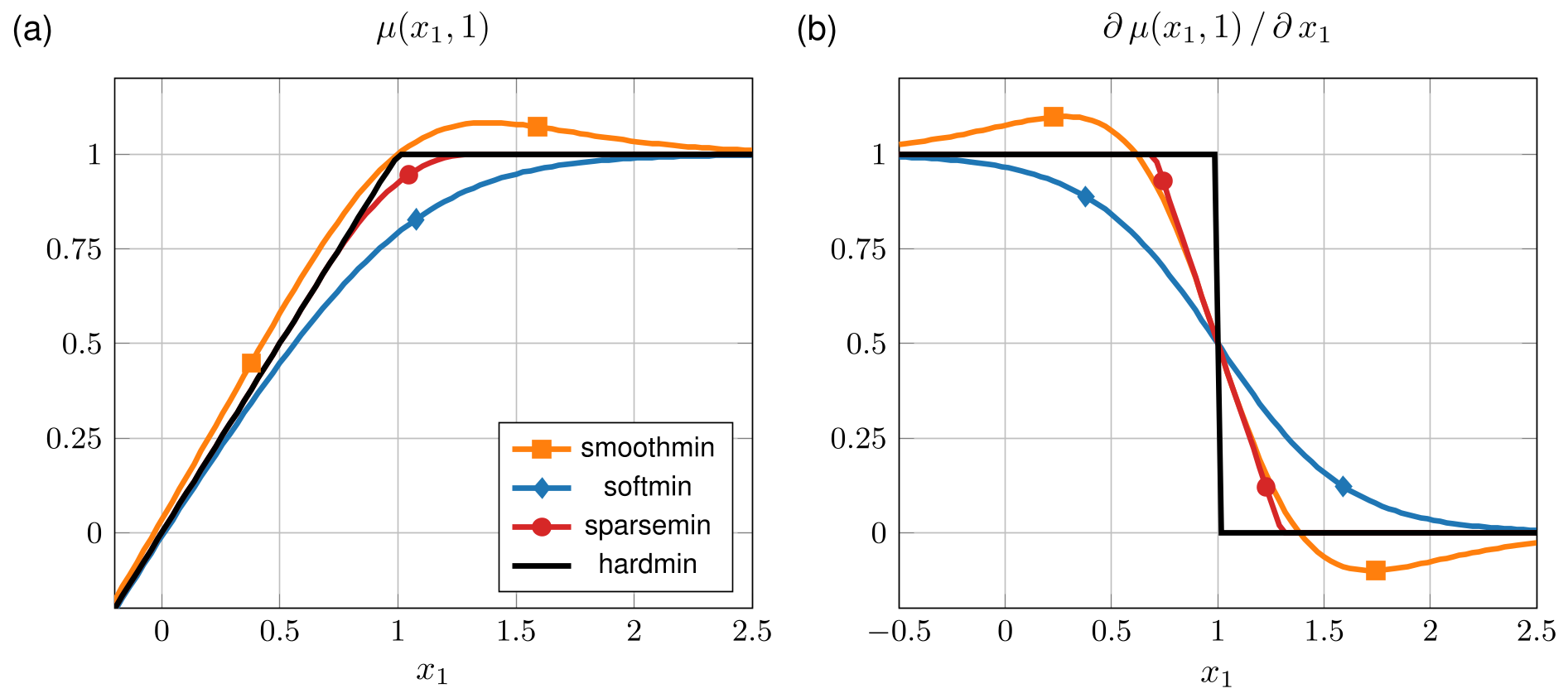
Minimum functions \(\mu\) and their partial derivatives.

Let \(\mu\) aggregate a finite vector of path costs \(v\in\mathbb{R}^D\). Important examples are the hard minimum

\[\mu_\mathrm{hard}(v)=\min_{d\in[1{:}D]} v_d\]

and the soft minimum

\[\mu_\mathrm{soft}(v) = -\gamma\log\sum_{d=1}^{D}\exp(-v_d/\gamma), \qquad \gamma>0.\]

The hard minimum selects a single lowest-cost path. The soft minimum performs a smooth log-sum-exp aggregation and assigns gradient mass in a probabilistic way. [3] The toolbox also includes smoothmin

\[\mu_\mathrm{smooth}(v)=\langle v, \nabla\mu_\mathrm{soft}(v)\rangle\]

and sparsemin

\[\mu_\mathrm{sparse}(v) = \min_{q\in\Delta^D} \langle v,q\rangle + \frac{\gamma}{2}\langle q, q-1\rangle\]

as differentiable variants. [4] [2] They can be used in the differentiable recursion but do not yield the same global path-aggregation equivalence that is guaranteed for hardmin and softmin. In the toolbox, choose among ("hardmin", "softmin", "smoothmin", "sparsemin").

Path-Prefix Cost

The aggregated cost \(\mathbf{D}(p)\) of all paths leading to a vertex \(p\) is

\[\mathbf{D}(p) := \mu\left( \left( w_\mathrm{start}^{p_1} +\sum_{\ell=2}^{L}\theta_{(p_{\ell-1},p_\ell)} \right)_{(p_1,\ldots,p_L)\in\mathcal{P}(p)} \right).\]

This quantity contains the start weight of the first vertex and all edge weights along the path prefix.

Alignment Loss

The full alignment cost aggregates all path-prefix costs that terminate at an allowed end vertex:

\[\mathcal{L}(X,Y) = \mu\left( \left( \mathbf{D}(p)+w_\mathrm{end}^{p} \right)_{p\in\mathcal{B}_\mathrm{end}} \right).\]

This is the mathematical loss represented by the forward() function of the dDTW module. Batch averaging and optional length normalization are applied afterwards.

Dynamic Programming Formulation

Enumerating all paths is infeasible because their number grows exponentially with sequence length. [5] Instead, dDTW computes \(\mathbf{D}\) recursively. Let

\[\Psi(p):= \{q\in\mathcal{I}\mid(q,p)\in\mathcal{E}\}\]

be the parent vertices of \(p\), and define

\[\begin{split}a(p)= \begin{cases} w_\mathrm{start}^{p}, & p\in\mathcal{B}_\mathrm{start},\\ \infty, & \text{otherwise.} \end{cases}\end{split}\]

Assuming that \(\mu\) ignores infinite alternatives, the forward recursion implemented in the toolbox is

\[\mathbf{D}(p) = \mu\left( a(p), \left( \mathbf{D}(q)+\theta_{(q,p)} \right)_{q\in\Psi(p)} \right).\]

Evaluating this recurrence over the DAG yields the accumulated cost matrix \(\mathbf{D}\in\mathbb{R}^{N\times M}\). The backward() function of dDTW executes the reverse dynamic program which computes gradients with respect to the local costs, and PyTorch then propagates these gradients further to the input tensors. [6] [7]

Summary: Toolbox Mapping

The general dDTW class exposes the graph components directly:

• cost_function or a precomputed \(C\) defines \(c(x_n,y_m)\).

• min_function selects \(\mu\).

• step_sizes defines \(\mathcal{S}\).

• global_step_weights and local_step_weights define \(\mathbf{W}\).

• B_start, B_end, start_penalty, and end_penalty define \(\mathcal{B}_\mathrm{start}\), \(\mathcal{B}_\mathrm{end}\), \(w_\mathrm{start}\), and \(w_\mathrm{end}\).

The predefined variants in ddtw.ddtw_variants fix these components for common objectives such as SDTW, subSDTW, partial_matching, and CTC.

References

[1]

J. Zeitler and M. Müller, “dDTW: A Unified and Efficient Toolbox for Differentiable Sequence Alignment,” submitted, 2026.

[2] (1,2,3)

A. Mensch and M. Blondel, “Differentiable Dynamic Programming for Structured Prediction and Attention,” in Proceedings of the International Conference on Machine Learning (ICML), Stockholm, Sweden, 2018, pp. 3459-3468.

[3]

M. Cuturi and M. Blondel, “Soft-DTW: a Differentiable Loss Function for Time-Series,” in Proceedings of the International Conference on Machine Learning (ICML), Sydney, NSW, Australia, 2017, pp. 894-903.

[4]

I. Hadji, K. G. Derpanis, and A. D. Jepson, “Representation Learning via Global Temporal Alignment and Cycle-Consistency,” in Proceedings of the IEEE/CVF Conference on Computer Vision and Pattern Recognition (CVPR), Virtual, 2021, pp. 11068-11077.

[5]

C. Banderier and S. Schwer, “Why Delannoy Numbers?” Journal of Statistical Planning and Inference, vol. 135, pp. 40-54, 2005.

[6] (1,2)

J. Zeitler and M. Müller, “A Unified Perspective on CTC and SDTW Using Differentiable DTW,” IEEE Transactions on Audio, Speech and Language Processing, vol. 34, pp. 936-951, 2026.

[7]

J. Zeitler and M. Müller, “Subsequence SDTW: Differentiable Alignment with Flexible Boundary Conditions,” in Proceedings of the IEEE International Conference on Acoustics, Speech, and Signal Processing (ICASSP), Barcelona, Spain, 2026.